Sierra Nevada Experiment (SNEP)

Many thanks to the SNEP group (G. Zandt, C. Jones, T. Owens, H. Gilbert, P. Crotwell, A. Frassetto).
More SNEP info HERE. Slides from recent seminar on SNEP results given by Dueker and Stachnik HERE.

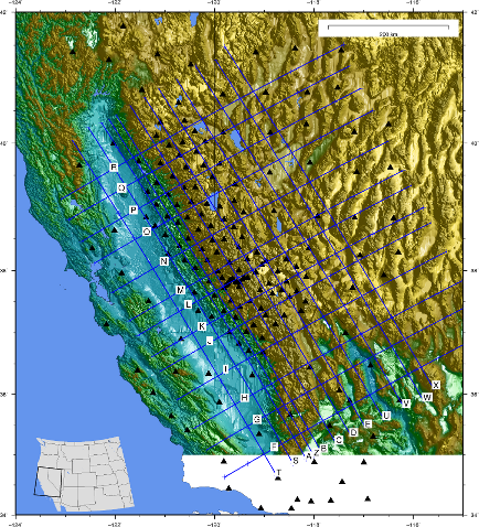
Preliminary shear velocity model from inversion of phase velocity dispersion measurements from ambient noise cross correlations (4-40 s) and two-plane wave analysis of teleseismic earthquakes (20-100 s, courtesy of Hersh Gilbert). The SNEP dataset has provided great results in comparison to others I have analyzed. This is the only dataset where the input starting model does not have a priori constraints on crustal thickness, yet upon inversion a Moho gradient is evident that is very sharp on the east side and less sharp on the west. This is largely due to the increased resolving power associated with the dense interstation spacing. PDF files for all images available below. Figure to left is a regional map showing stations and cross section locations. PDF 2.1MB

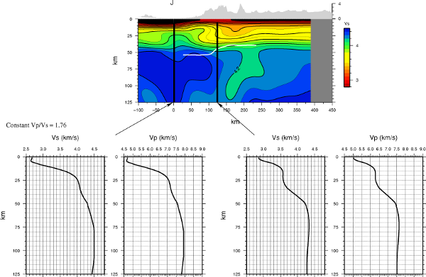
Shear velocity cross section J. Solid white line indicates approximate Moho depth from interpolated map of crustal thickness from receiver functions (Frassetto et al., in review).

Determination of Crustal Thickness from gradient analysis of shear velocity profiles:
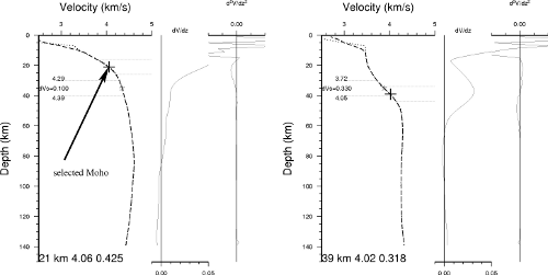
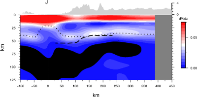
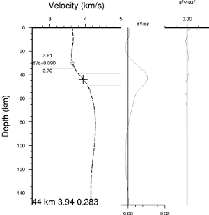
The numerical first derivative was calculated for each 1D Vs profile. The Moho was automatically selected to be the maximum of the first derivative between 20 km and 60 km depth, with a Vs>4.0 km/s. Below are example profiles, similar to those above. The automatically selected Moho is shown by the "+" in the velocity profile. In the first example for a profile beneath the western foothills, the high velocity lower crust makes determining the Moho difficult in this manner as the largest velocity gradient occurs in the upper 15 km. The cross section below shows the shear velocity gradient for cross section J. The black dashed line indicates the Moho from receiver functions (Frassetto et al.) and the black dotted line is the inferred Moho from the shear velocity gradient analysis. The black region is where the gradient < 0.

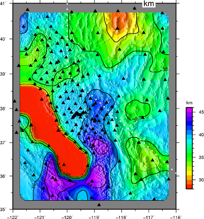
Crustal Thickness map:

Crustal thickness map from velocity gradient analysis. Crustal thickness beneath the Great Valley is probably selected incorrectly (see leftmost velocity profile above) so image is clipped at 28 km which is why the Great Valley is all red.

Velocity gradient cross sections obtained here:
EW cross sections (PDF, 200Kb)
NS cross section (PDF, 200Kb)

Testing Velocity Discontinuity (Moho) resolution:

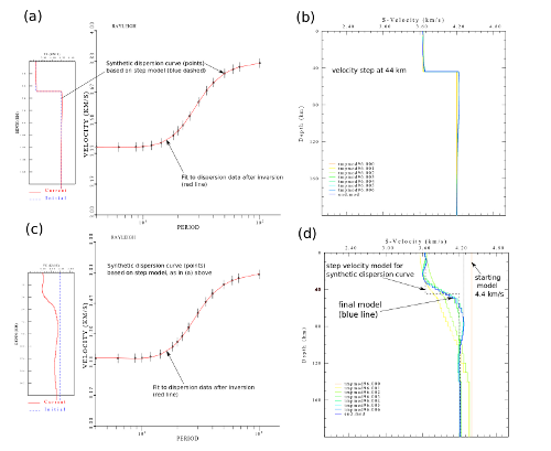
This is the simplest, and probably end member test that shows inverting the dispersion measurements alone cannot resolve a discrete discontinuity in the velocity model, but the mean of the system can be captured, i.e. the Moho depth as the inflection point of the velocity gradient.

(a) created a synthetic dispersion curve based on a velocity model that increases in shear velocity from 3.65 km/s to 4.2 km/s at 44 km depth.

(b) inverted dispersion data for shear velocity using the same input model as the starting model for the inversion. Clearly, the input model was recovered as expected.

(c) Using the same synthetic dispersion curve, the inversion was performed with a uniform starting model at 4.4 km/s

(d) The final model (blue line) captures the average of the input model (dashed line) and the Moho corresponds to the inflection point of the velocity gradient in the appropriate depth range. Also, the maximum shear velocity reached below the Moho at about 75 km depth overestimates the real velocity by about 0.075 km/s (vertical dotted line). This overestimation is likely the highest possible since this synthetic test uses a 0.55 km/s jump at the Moho, where beneath SNEP the velocity jump is closer to 0.4 km/s.

The inversion of the synthetic dispersion curve was performed with the same damping, smoothing, and number of iterations as was used for the full SNEP inversion.

The velocity gradient analysis was performed using the final model from the above synthetic inversion (blue line in (d) above). From the peak in the first derivative of the velocity profile, a Moho depth of 44 km was retrieved. This is exactly as the input model from which the synthetic dispersion curve was created.

PDF files:
SNEP Talk (26MB)
Shear velocity Cross section J above (50k)
Regional map (2.1MB)
East-West shear velocity cross sections (400kB)
North-South shear velocity cross sections (400kB)
Shear Velocity Depth slices (58MB) - note color palette changes at 40km depth
Notes:
* 0 km locations on cross sections are same as in the recently submitted Frassetto et al. paper.
* Solid white line on cross sections indicates approximate Moho depth from interpolated map of crustal thickness from receiver functions
* 1-D inversions for shear velocity performed with uniform starting model. Future work to include joint inversion with receiver functions from Frassetto.

Processing:
1) 2-D phase velocity maps were constructed from interstation phase velocity measurements (4-40 s)
2) 2-D phase velocity maps from two-plane wave analysis of teleseismic earthquakes by Hersh Gilbert (20-100 s)
3) Phase velocity maps sampled on 0.1 degree grid, to create a dispersion curve at each grid node
4) 1-D inversion for shear velocity at each grid node using a uniform 4.4 km/s starting model

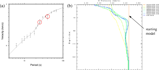
Example of dispersion curve (a) and resulting velocity model after 6 iterations (b). Red circles in (a) show overlapping phase velocity observations from ambient noise and two-plane wave.

Model regularization:

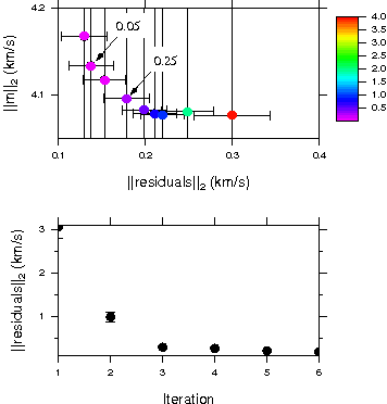
Although the L-curve analysis of general inverse problems is a heuristic, it provides a quantitative approach to the trade-offs. As this is an iterated least-squares problem, the bottom plot below shows that with a few iterations the L-2 norm of the residuals decreases rapidly and the solution converges. The upper plot shows the characteristic L-curve between the L-2 norm of the residuals and the L-2 norm of model (model energy) for different damping parameters (color-coded) after 6 iterations for grid nodes in the central Sierras. Two particular damping parameters are noted (0.05 and 0.25). The model with damping of 0.05 is preferred because the resulting model reveals velocity structures and gradients more consistent with prior knowledge, in particular the negative velocity gradients found at about 80 km depth in the Frassetto Pds work and the recent Abt et al. work with Sdp. Also, the mid crustal low velocity region under the north Owens Valley/Long Valley volcanic field is evident.

Future Model Tests:
1. Compare predicted teleseismic body wave S arrival times to model predictions
2. use Yosemite dense line to test Moho gradient predictions
3. Carefully look for some Sdp arrivals to test for base of lid.

Feature Recovery Tests:
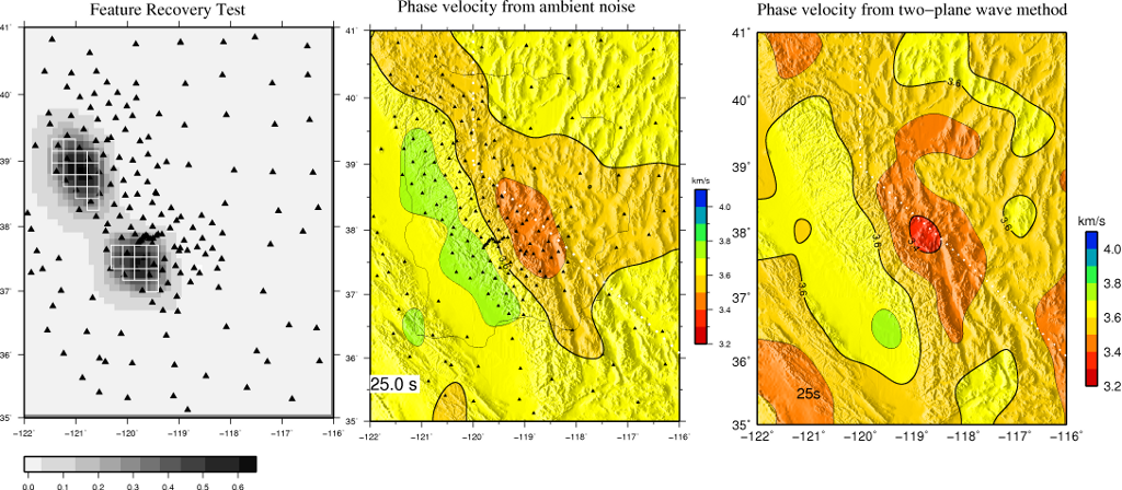
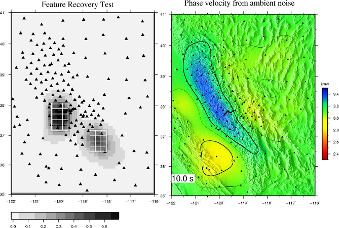
I prefer "feature recovery" tests over traditional checkerboard tests because they represent more realistic anomalies than the oscillatory pattern in a checkerboard. Plus, checkerboard tests never look as nice as I would like. These tests show good recovery of distinct anomalies at these periods.

Here is an example at 25 s period. The input model is unity in amplitude and outlined by the white lines. The colored gray scale shows the recovered model. The middle panel is the phase velocity map at 25 s from ambient noise cross correlations and the third panel is the phase velocity map from the two-plane wave method. The maps are very similar for the two different methods, with the ambient noise having higher resolution.

Another example at 10 s period:

Raypath Density:

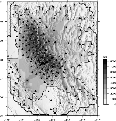
Below is a map at 10 s period showing the total length of raypaths in each of the 20 km x 20 km blocks in the ambient noise phase velocity tomography. The contours are only drawn at 0, 500, 1000 km, inside of which the length of raypaths increases rapidly as shown by the color scale. Maps at other periods show a similar pattern.

Velocity Resolving Kernels:

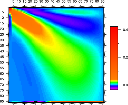
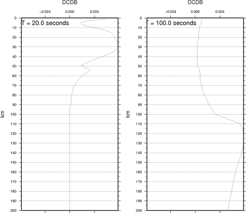
The image below shows the velocity resolving kernels for a typical 1D well inversion for shear velocity. The axes are model parameter number, which in this case are 0.5 times the depth since the model is parameterized with 2 km thick layers. The color palette is saturated, but shows that at 80 km depth the resolution becomes about half of the maximum value. With dispersion measurements out to 100 s, we still have sensitivity beyond 80 km, but the partial derivatives dC/dB (change in phase velocity with change in shear velocity) are much broader (see below).

Partial Derivatives for shear velocity inversion:

Example partial derivatives dC/dB (change in phase velocity with change in shear velocity) for 20 and 100 s periods, calculated for a velocity model with Moho at 42 km depth.